ABSTRACT
To precisely quantify pore space and organic matter (OM) from two-dimensional scanning electron microscope (SEM) images, an efficient and consistent workflow using adaptive local thresholding, Otsu thresholding and Image Calculator are presented. It can offer an automated segmentation of pore space and OM, then differentiates the porosity hosted by OM and minerals. The workflow is demonstrated on a widely distributed set of core samples from Mahantango and Marcellus shale units of the Appalachian basin. The vitrinite reflectance of these samples ranges from 1.36% to 2.89%, covering a spectrum of thermal maturity. Organic matter abundance and mineralogy also vary significantly. The results are compared with routine rock property tests, such as helium porosimeter (Gas Research Institute method), and total OM. The proposed workflow improves quantitative determination of porosity above a certain pore size and OM in shale samples. Advantages of this workflow include improved consistency and speed of analysis of SEM images of shale samples at the nanoscale.
INTRODUCTION
The exploration and exploitation of shale gas reservoirs have attracted global interest in this fine-grained rock type. Shale gas production in the United States increased from 0.8 tcf (22.7 billion m3) in 2000 to 15.7 (444.6 billion m3) tcf in 2016 and will account for nearly two-thirds of natural gas production by 2040 (US Energy Information Administration, 2017). Porosity, pore structure, organic matter (OM) abundance, grain assemblage composition, and thermal maturity are key factors in assessing shale gas resources and reserves and understanding storage capacity and long-term producibility of a shale gas reservoir. Shale, or more correctly, mudrock (mudstone), has long been considered as seal or source rock because of its low permeability and tendency to be associated in the geologic record with preserved OM (Zagorski et al., 2012).
One aspect that makes a mudrock reservoir “unconventional” is that conventional drilling and completion technologies are not successful in hydrocarbon production because of the nanoscale pore sizes. Characterization of nanometer pores in a mudrock reservoir requires a high-resolution technique to show the fine-scale properties. Compared with other technologies, such as mercury injection capillary pressure, physical adsorption, nuclear magnetic resonance, and helium porosimeter, scanning electron microscopy (SEM) provides a direct visual observation of the complex microstructure of a mudstone reservoir, which has good potential to decipher the heterogeneity of pore size and geometry and grain assemblage (Dilks and Graham, 1985; Katz and Thompson, 1985; Jarvie et al., 2007; Loucks et al., 2009, 2012; Ross and Bustin, 2009; Schieber, 2010, 2013; Sondergeld et al., 2010a; Curtis et al., 2011, 2012; Slatt and O’Brien, 2011, 2013; Walls and Sinclair, 2011; Fishman et al., 2012; Klaver et al., 2012, 2015, Milliken et al., 2012, 2013, 2014; Passey et al., 2012; Bohacs et al., 2013; Dong and Harris, 2013; Driskill et al., 2013; Giffin et al., 2013; Pommer and Milliken, 2015; Saidian et al., 2015; Milliken and Olson, 2016; Nole et al., 2016; Schieber et al., 2016). It can also illustrate the distribution of resolvable porosity associated with OM and minerals. Quantification of nano- to microporosity and pore structure is important for evaluating the storage capacity and flow regime in unconventional reservoirs (Javadpour, 2009; Sondergeld et al., 2010b).
Scanning electron microscopy has been exploited in various industries because of its potential high magnification and ability to resolve fine-scale features. Unlike optical microscopy, SEM uses an electron beam to scan the sample surface, and it generates images by recording the interaction of the electron beam with atoms of the specimen at various depths within the sample. Several types of electrons carrying distinct structural and compositional information are generated (e.g., secondary electrons [SE], backscattered electrons [BSE], etc.), and they differ from one another in origin, energy, and travel direction (Huang et al., 2013). Type I SE (SE1) are generated at the point of primary electron beam with a high angle that allows them to carry surface topographic information with the highest resolution. Type II SE (SE2) are generated when BSE leave the surface of the specimen at a lower angle. Type II SE add atomic number contrast to the SE image, which reveals both topographical and compositional information. The interaction volume of BSE is much deeper than SE. A backscattered electron signal depends on the atomic number; therefore, it contains more compositional information. (Huang et al., 2013).
Improved physical processing of samples has provided a significant improvement in SEM analysis of mudrock. With mechanical polishing, quantitative analysis of shale is nearly impossible because numerous artificial pores are created because of sample breakage (Loucks et al., 2009). The ion milling technique uses a beam of ions to very precisely mill a sample. By carefully controlling the energy and intensity of the ion beam, a surface that is flat at the nanometer scale is produced, resulting in removal of topographic artifacts and producing clearer imaging of pore structures and mineral textures (Erdman and Drenzek, 2013), which sheds new light on the nanoscale microstructure and evolution of pores contained within the OM and inorganic mineral matrix of mudrock reservoirs (e.g., Loucks et al., 2009, 2012; Ambrose et al., 2010; Sondergeld et al., 2010a, b; Curtis et al., 2011, 2012; Slatt and O’Brien, 2011; Milliken et al., 2013, 2014). However, ion milling can create some artifacts, such as curtain effects, and redeposition of milled minerals. Other artifacts include mineral precipitation after sample preparation and postcoring precipitations (Milliken and Olson, 2016). Most of these artifacts are easy to recognize (Loucks et al., 2012; Anovitz and Cole, 2015; Milliken and Olson, 2016). Nole et al., (2016) published a method to circumvent the artifacts created during ion milling using the differences in circularity values in a segmented image.
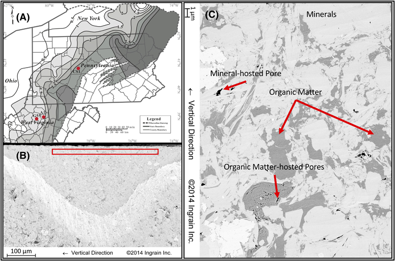 Figure 1. (A) Locations of the three study wells. Contours depict regional averages of vitrinite reflectance (modified after Zagorski et al., 2012 and used with permission of AAPG). (B) Overview of the ion-milled region and scanning electron microscopy (SEM) area; the red rectangle indicates the locations of the smaller field of view SEM images, notice the stringers of organic matter (OM) were avoided. (C) Sample type II secondary electron SEM image illustrating major rock facies (high density minerals, OM, and pore space) seen in SEM image of shale. The remainder of the image is the inorganic mineral matrix of mudrock, which typically has a density between 2 and 3 g/cm3.
In SEM (especially SE1 or SE2) images, pore space is defined by very low grayscale values (dark), whereas minerals’ surfaces have higher grayscale values (Hemes et al., 2013; Figure 1). Thresholding and segmentation of pore space and OM from SEM images are the beginning of quantitative image analysis, yet they are challenging on shale samples because the process of image segmentation does not necessarily lead to unique solution. On the one hand, the variation of instrument settings can cause grayscale level shift from some images to others. Even within a single image, the characteristic grayscale value of OM, minerals, and pores can vary (Anovitz and Cole, 2015; Figure 2). In addition, imaging artifacts, especially edge effects at pore boundaries, make it hard to choose an appropriate segmentation algorithm (Kelly et al., 2016).
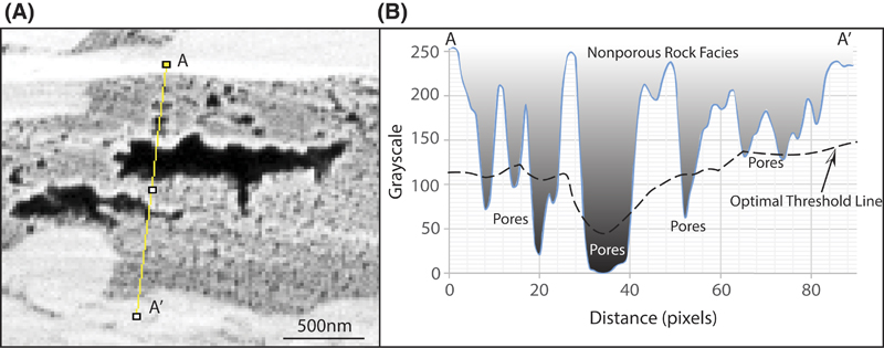 Figure 2. (A) A sample image featuring the local variance of grayscale of pores. (B) Grayscale profile of AA′, the dashed line is the optimal threshold line. Notice the optimal threshold changes along the profile. The location of AA′ is shown in (A).
Image segmentation is the process of partitioning an image into several separate regions. Thresholding is a simple method for image segmentation (Zhang et al., 2008). All pixels with grayscale values above (or below) the threshold value are assigned to a particular class, such as OM. More than one way exists to seek an appropriate thresholding method to segment a two-dimensional (2-D) image (or a three-dimensional [3-D] volume). One method is manual thresholding, in which the operator searches the whole range of grayscale (for an 8-bit image, the range is from 0 to 255) and find a specific threshold that contains most of the foreground pixels. Zhang et al. (2011) explored the lack of consistency with manual thresholding by systematically studying the effect of different thresholds on the pores. They test a grayscale range from 10 to 100, and set 45 to 65 to be the range that gave reasonable results. But even within this reasonable range, the estimated porosity ranged from 4% to 13% (Zhang et al., 2011). Automated thresholding is preferable not only because it saves time, but it also helps eliminate human bias or subjectivity by increasing consistency (Wildenschild and Sheppard, 2013). Hemes et al. (2013) used a combination of thresholding and Sobel edge detection algorithms to segment the pores, then used Esri ArcGIS (geographic information system software) to manually correct the inaccurate pore segmentations (also Klaver et al., 2015). This methodology involves a large amount of manual correction of the segmentation, so it is very time intensive when dealing with large SEM images. Kelly et al. (2016) employed a comprehensive image analysis workflow. They compared two different image segmentation methods. One is a fuzzy-logic, membership function–based, c-means centroid search “soft thresholding.” The other is histogram-based thresholding with implementation of a level set method. In many cases, the level set contours caused overestimation of the OM-hosted porosity. Neither image segmentation method provided large enough connectivity. A consistent, efficient, and trackable method of image analysis with high accuracy is very much needed for nanoscale porosity typical of mudstones.
Sezgin and Sankur (2004) reviewed 40 different image thresholding methods and classified them into 6 categories based on the information they exploited: histogram shape, clustering, entropy, object attribute, spatial methods, and local methods. Among all these methods, for SEM images of rock samples, Zhang et al. (2011) recommended using top-hat segmentation. This algorithm picks up a peak or valley based on a local criterion. Yet, a threshold still needs to be chosen, and for the reasonable grayscale range discussed above (from 45 to 65), the porosity results varied from 7% to 3.5%. Because of the local variance we noticed in our images (Figure 2) and in a large number of images that have been published over the years, we hypothesize that local thresholding that adapts the threshold value on each pixel to the local image characteristics (Sezgin and Sankur, 2004) is more promising than global thresholding.
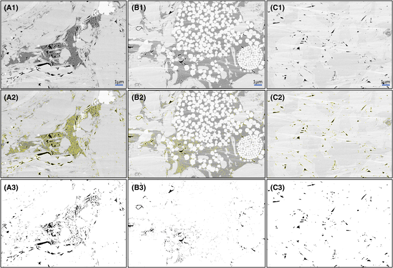 Figure 3. Illustration of the pore segmentation on test sample (A) (from well CS1, 7133.75 ft [2174.37 m], Marcellus Shale), (B) (from well G55, 7162.45 ft [2183.11m], Marcellus Shale), and (C) (from well A1, 7620.10 ft [2322.61 m], Mahantango Formation). (A1–C1) Original images. (A2–C2) Manually picked results with yellow outlines highlight the pore border. (A3–C3) Automatic thresholding results using the proposed method.
Currently, no standard workflow exists for acquiring petrophysical properties (e.g., porosity and OM richness) from SEM images of organic-rich shale. We introduce a workflow for quantitative SEM image analysis that improves consistency and efficiency of results, and we demonstrate the applicability of the workflow for investigating pore structure and OM character. The resulting quantification can contribute to improving our knowledge about heterogeneity of pore systems and OM in mudrock and other fine-grained rocks and to better understand heterogeneity’s factor in controlling the reservoir properties in oil and gas exploration and production. Pore size and type distribution are also associated with facies and sequence stratigraphy position as well as fabrics.
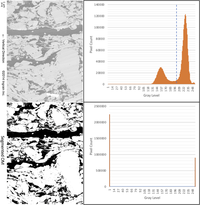 Figure 4. Illustration of applying Otsu thresholding to segment the organic matter (OM). Grayscale histograms are listed next to the original image and segmented OM. The blue dash line indicates the postulated optimal segmentation strategy. Two clusters in the histogram of the original image represent the OM and the mineral matrix. This bimodal distribution of grayscale makes it feasible to segment the image with Otsu thresholding.
Critical questions to address in quantitative image analysis of organic-rich mudrock are the following: (1) how to choose a nonbiased threshold to segment pore space and OM from SEM images and (2) how to separate OM-hosted pores from the whole-pore system? These questions illustrate a common challenge associated with image analysis: reproducibility, commonly addressed subjectively by the operator, but can be subject to bias and inconsistency. We test this workflow with our own samples and an image donated by Guochang Wang from St. Francis University by comparing our results with a reference data set derived from manual pore picking from the same images.
DATA AND METHODS
Data for this research consist of 32 core samples collected from 3 wells penetrating the Mahantango Formation and Marcellus Shale in the Appalachian basin (Figure 1A). Samples range in depth from 7015.00 to 7778.15 ft (2138.17 to 2370.78 m). For this study, the core samples were ion polished at Ingrain’s Digital Rock Physics Lab with Gatan Ilion+ argon ion polishing system. No conductive coatings were applied to the milled surfaces. An area that is approximately 1 mm by 500 μm is polished (the roughly triangular area in Figure 1B). A 2-D SEM overview image is taken with a field of view of approximately 750 μm (Figure 1B). The red rectangle within the overview indicated where the smaller field of view 2-D SEM separate images were acquired (Figure 1C). Approximately 10 locations per sample were imaged with Carl Zeiss SEM systems at a low beam energy of 1 kV. Both BSE and SE2 detectors are used to capture separate images. Images from well A1 and G55 are taken at resolution of approximately 15 nm/pixel, whereas images from well CS1 are taken at resolution of 10 nm/pixel (e.g., Figures 3–5). All samples were viewed perpendicular to bedding (Figure 1C). Type II SE SEM images are used in this research. The SEM images were processed with ImageJ and Fiji (Schindelin et al., 2012, 2015; Schneider et al., 2012). Median filter with a radius of two pixels was applied before quantification to reduce the noise in the images (Gallagher and Wise, 1981; Culligan et al., 2004, 2006; Kelly et al., 2016; Nole et al., 2016).
 Figure 5. Illustration of the organic matter (OM) segmentation on test sample (D) (from well G55, 7201.10 ft [2194.90 m], Marcellus Shale), (E) (from well CS1, 7136.85 ft [2175.31 m], Marcellus Shale), and (F) (from well A1, 7729.50 ft [2355.95 m], Marcellus Shale). (D1–F1) Original images. (D2–F2) Manually chosen results with blue outlines indicating the OM border. (D3–F3) Automatic thresholding results using the proposed method.
The surface of shale sample shown in Figure 6 was prepared by an argon ion polisher with a Jeol IB-09020CP and coded with platinum. The images were acquired by concentric backscattered detector using an FEI Helios NanoLab 600i field-emission SEM. The working distance is 3.3 mm, and the image was taken at an accelerating voltage of 8 kV.
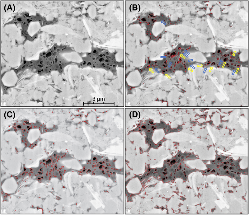 Figure 6. Application of the proposed workflow on an independently supplied image. (A) Original image; (B) automated pore segmentation with red outlines highlighting the border of pores, yellow arrows depict the low-angle deepening pore border, and blue arrows depict the difference between manual and automated segmentation; (C) pores manually segmented by an independent third party; and (D) automated segmented organic matter. Image courtesy of Guochang Wang.
Total organic carbon (TOC) content was quantified using the source rock analyzer, and the results were expressed in weight percentage. Approximately 60 to 100 mg of pulverized rock was analyzed. Free hydrocarbons (S1) and hydrocarbons result from thermal cracking of nonvolatile OM (S2) are quantitatively detected and reported as milligrams of hydrocarbon per gram of rock. The free CO2 (S3) produced during pyrolysis of kerogen is reported as milligrams of CO2 per gram of rock. Residual carbon (S4) is also measured and reported as milligrams of carbon per gram of rock. Total organic carbon is calculated by %TOC = 0.1 × (0.082 × [S1 + S2] + S4) (Espitalie et al., 1985). Organic matter abundance values in volume percent is the volume percent of OM calculated from the bulk TOC (weight percent) by assuming an OM density of 1.45 g/cm3 (Milliken et al., 2013).
Image Analysis Workflow
We illustrate a workflow that automatically thresholds an SEM image by adaptive local thresholding (Phansalkar thresholding) and Otsu thresholding. Then, a methodology is presented to further segment porosity between OM and mineral matrix by Image Calculator. All steps are undertaken with Fiji, which is an open-source software developed by the National Institutes of Health. Every step of the methodology is trackable, so it offers not only a final numeric result, but also precision and repeatability. The methodology is a step toward establishing a consistent and objective numerical model of the visible nanoscale pore structure of mudrock observable in SEM images. Results demonstrate that this method is highly efficient and provides a high degree of precision and repeatability in image processing, advancing the study of pore structure of mudrock.
Segmentation of the Pore Space
Thresholding is the first and most important step of image segmentation to discriminate and quantify pores versus matrix. The process of image thresholding does not necessarily yield a unique solution for a threshold. The main reason is variation in illumination level resulting from different voltage of current, or simply caused by different instruments, in which case, a single type of rock component (e.g., OM) will show different absolute grayscale ranges. Therefore, a universal thresholding system is unlikely to exist, and selecting an appropriate method to find thresholds is of great significance. Because humans cannot distinguish different grayscales consistently, choosing thresholds manually introduces subjectivity and uncertainty because of the lack of consistency between operators, and even between instances for the same operator (Anovitz and Cole, 2015).
To address this challenge, we recommend adaptive local thresholding. Sauvola and Pietikainen (2000) published a method that determines a local threshold for each pixel based on local variance and standard deviation. This method was originally designed for document analysis. When uneven illumination or stains exist, global thresholds cannot offer consistent results (Sauvola and Pietikainen, 2000). In certain areas, the grayscale of pores is equal to that of OM in other areas, which causes significant error when trying to quantify the porosity (Figure 2). The abovementioned local variance is largely caused by “shallow dipping of a pore boundary” (also known as pore backs [Canter et al., 2016, p. 21]), which results in low grayscale gradients in a certain region (Hemes et al., 2013). The optimal threshold strategy is to determine a local threshold for each pixel based on local variance as demonstrated in Figure 2A, B. Phansalkar et al. (2011) applied this method to cytological image analysis and noticed a problem. When the contrast in the local neighborhood is very low, the relatively dark regions will be removed (categorized as background). In cytological (SEM) images of shales, these dark regions are also foreground. They fixed this problem by using a new equation to calculate the local thresholds
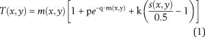
in which T(x,y) is the local threshold, m(x,y) is the mean, s(x,y) is the standard deviation, and k equals 0.5, p equals 2, and q equals 10 (Phansalkar et al., 2011).
When applying adaptive local thresholding, the operator needs to choose a window size. It gives a limit of the region within which the local threshold will be computed with local adaptive thresholding. When the radius is too big, it will operate the same as global thresholding. Whereas when it gets too small, the local variance will be enhanced and makes it harder for the pores to be discriminated from the rock matrix. Sauvola and Pietikainen (2000) recommend to set the window size to 10 to 20 pixels (Sauvola and Pietikainen, 2000). Figure 3 shows the result of manually picked pores versus automated segmentation.
Segmentation of the Organic Matter
Otsu’s method is used to threshold OM and pore space. This method was developed by Nobuyuki Otsu in 1979 (Otsu, 1979), and it automatically performs clustering-based image thresholding. It reduces a grayscale image to a binary image. The algorithm assumes that the image contains two classes of pixels that are distributed in a bimodal histogram (foreground pixels and background pixels). Foreground pixels are the OM and background pixels are the mineral matrix. The optimum threshold is established by minimizing the weighted sum of intraclass variances of the foreground and background pixels, or equivalently (because the sum of pairwise squared distances is constant), maximizing the interclass variance (Figure 4).
The intraclass variance is defined as a weighted sum of variances of the two classes.

Weights ω0,1 are the probabilities of the two classes separated by a threshold, t and  , are variances of these two classes. One of the two classes is the darker part of the image, which is OM and pore space. The other class is the rest of the input image, which is minerals. Because we already have the pore space segmented by now, it can be subtracted from the Otsu thresholding result with the Image Calculator feature in Fiji or ImageJ, and the OM remains. Figure 5 shows the result of manually picked OM versus Otsu thresholding.
Determining Porosity Associated with Organic Matter and Minerals
The OM-hosted porosity in organic-rich shale reservoirs is formed during thermal maturation of OM (e.g., Loucks et al., 2009, 2012; Schieber, 2010, 2013), which is of great significance in evaluating the reservoir and understanding the evolution of pores in shale (e.g., Milliken et al., 2013). Loucks et al. (2012) summarized classification of pore types in shale and present a self-explanatory classification system featuring interparticle, intraparticle, and OM pores. Milliken et al. (2013) studied the Marcellus Shale and subdivided OM pores into three types. Pommer and Milliken (2015) further defined OM–mineral interface pores as pores between mineral particle and OM and categorized this as mineral-associated rather than OM-hosted pores. In this research, we will follow the Pommer and Milliken (2015) classification.
Other than picking pores manually, a detour can be taken. If the pores within segmented OM (e.g., Figure 5D3, E3, F3) can be digitally infilled, the percentage of OM plus OM-hosted porosity in the image can be determined. The infilled OM can be subtracted from the total pore space map (e.g., Figure 3A3, B3, C3) with Image Calculator. The Image Calculator function of ImageJ assumes that subtracting a value (infilled OM) from a null value will result in a null value. Because no OM exists on the total pore space map after the subtracting, there will only be pores that are not hosted by OM. The OM parts will remain as null value. The result is the mineral-hosted porosity. The OM-hosted porosity is simply determined by subtracting mineral-hosted porosity from the total porosity.
When trying to infill the void space in OM, several different cases exist. The ideal case is pore space fully enclosed within OM. This type of OM-hosted pore can be directly filled with the Fill Holes feature of Fiji or ImageJ after the OM is segmented. Another case is pores located very close to the border of OM, which, after segmentation, is not fully enclosed in OM. For this type of pores, we recommend using the Dilate feature in Fiji or ImageJ to add pixels to the edges of OM. By doing so, the gap of open borders of OM can be connected. After that, run Fill Holes and Erode (another feature of Fiji or ImageJ) to remove the same amount of pixels from the edges (Figure 7). This operation can also compensate the bright ring created because of the topographical artifact and mineral edge charging.
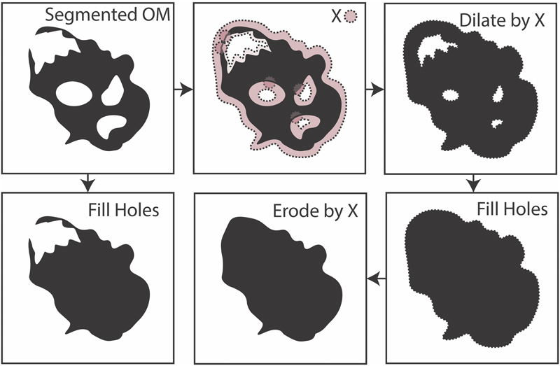 Figure 7. Processes of filling pore space within segmented organic matter (OM). The X symbol stands for the radius of dilation. Pores fully enclosed by OM can be filled directly. For OM that has pores on the edge, it needs to go through Dilate by X (number of pixels), Fill Holes, then Erode by X. The infilled pores will not be affected by the erosion. The demonstration is not associated with a specific scale because it can be applied to a range of scale.
To summarize, a 2-D grayscale SE2 SEM image undergoes automatic thresholding and segmenting into several rock components. Next, segmented binary images of pore space and OM are produced. Then, OM is digitally infilled. With Image Calculator, the infilled OM is subtracted from the total pore space map to generate the mineral-hosted pore space map. Mineral-hosted pores can then be subtracted from total pore space to generate OM-hosted pore map. The percentage of each rock components (OM, OM-hosted porosity, mineral-hosted porosity, and total porosity) can be calculated by Particle Analyzer in Fiji or ImageJ. Subsequent statistical measurements can be applied to each component, such as equivalent circular diameter, pore width, and circularity (supplementary material available as AAPG Datashare 107 at www.aapg.org/datashare).
RESULTS
Figure 3 demonstrates the porosity segmentation results of three samples. Sample A comes from well CS1 and features SE2 image with a substantial backscatter component so that the contrast between minerals, OM, and pores is very vivid. The pore system is a combination of both OM-hosted and mineral-hosted pores. Sample B comes from well G55, and most pores in this image are within OM. Sample C comes from well A1, and the pore system is mostly mineral-hosted pores. Most of the pores are formed by the chaotic stacking pattern of clay particles. Figure 3A2, B2, and C2 shows the manual picking results, with yellow lines highlighting the pore borders. Figure 3A3, B3, and C3 shows the automatic thresholding results. To reduce the effect from noise, the minimum pore size analyzed in this research is a three-by-three cluster of pixels (McCoy, 2005), which represents 30 nm in CS1 samples and 45 nm in A1 and G55 samples.
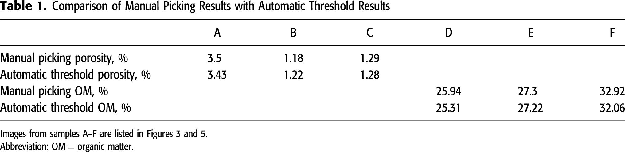
Figure 5 shows the results of OM segmentation in samples D, E, and F. Figure 5D2, E2, and F2 shows manual picking OM with blue lines highlighting the OM borders. Figure 5D3, E3, and F3 shows automatic thresholding results. The manually picked results are listed as a reference data set in this research, although we have to admit the fact that quantification of SEM images of shales can hardly lead to a result that can be used as ground truth because of multiple reasons we discussed earlier in this paper. The result is compared with TOC in weight percent. Richness of OM from image analysis has a strong positive correlation with TOC. The comparison of automatic threshold result with the reference data set (manual pick result) is listed in Table 1.
We also tested one image from a Chinese shale sample, which was donated by Guochang Wang from St. Francis University. The result is demonstrated in Figure 6.
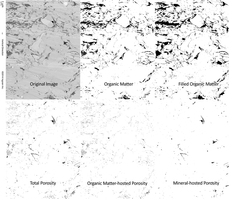 Figure 8. Segmentation results of a test image illustrating organic matter, filled organic matter, total porosity, organic matter–hosted porosity, and mineral-hosted porosity (test image from well CS1, 7114.50 ft [2168.50 m]). Quantification can then be applied to each segmented rock facies.
Figure 8 illustrates the result of separating OM-hosted porosity and mineral-hosted porosity by the proposed workflow.
DISCUSSION
Sensitivity Test
We conducted a sensitivity test on the effect of the thresholding parameter on the pore segmentation result, using samples A, B, and C. The local threshold window radius was tested in a range from 10 to 20 pixels (Figure 9). For sample A, we observed a gradual increase of the porosity result from 3.18% to 3.63% when the local threshold window radius increases from 10 to 20. They showed a very good linear correlation. For sample B, the porosity increases from 1.09% to 1.33% in the same window range. Sample C shows a different trend. The porosity readings at 10-, 15-, and 20-pixel window radii are 1.26%, 1.28%, and 1.27%, respectively. The porosity change is negligible, which indicates that thresholding window radii do not affect segmentation results in sample C case. This helps explain the very low coefficient of determination (R2) value of sample C in Figure 9. Based on this observation, if we choose 15 pixels as the thresholding window radius, then for sample A, the porosity in a 10- to 20-pixel window changes within 0.25%. For sample B, the porosity value changes approximately 0.12%. The consistency of the adaptive local thresholding is assumed to be acceptable and is completely repeatable if using the same window size on the same image. The manually picked results for these three samples are 3.50%, 1.18%, and 1.29%, respectively. We recommend choosing 15 pixels as the default local threshold window radius, because for samples A and B, it produces the median value of porosity so that the variance in result is minimized. On sample C, the result is not very sensitive to the radius setting. By setting the window radius to a fixed number, we can reach a consistent result.
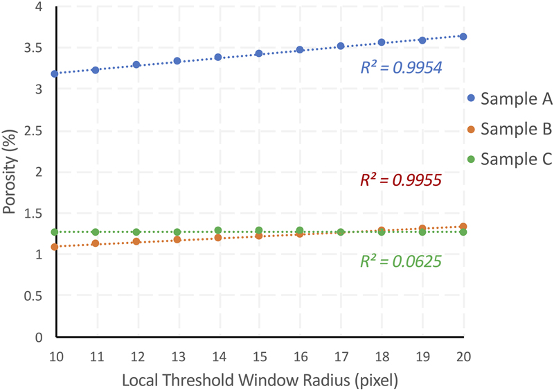 Figure 9. Sensitivity test of local threshold window radii and segmentation result (porosity). R2 = coefficient of determination.
All three samples we used to demonstrate the method are SE2 SEM images, but their pore types are different. In sample C, most of the pores are hosted by clay particles. The contrast between pores and minerals is very vivid, in which case, the porosity readings are very similar through different thresholding window radii.
We also tested the effect of image resolution. The original images were saved as 600 pixels per inch (PPI). We change the resolution by reducing the pixel density and then run the segmentation automatically and manually. We tested 300, 100, and 75 PPI. For wells A1 and G55 (original resolution 15 nm/pixel), these changes represent an analysis of 30 nm/pixel, 90 nm/pixel, and 120 nm/pixel, respectively. For well CS1 (original resolution 10 nm/pixel), these changes represent an analysis of 20 nm/pixel, 60 nm/pixel, and 80 nm/pixel, respectively. Although each sample trend is different, we observe an overall decrease in porosity results when reducing the input image resolution (Figure 10). For example, in reducing the resolution from 600 to 300 PPI, samples A, B, and C lost 0.36%, 0.51%, and 0.21% visible porosity, respectively, by automatic thresholding, and 0.49%, 0.30%, and 0.07% visible porosity, respectively, by manual picking. This change is much higher than the effect of threshold window size. Also, we notice that the visible porosity loss of sample C is lower than the other two samples. We attribute this to the fact that sample C has the least OM content, which makes the pores easier to be picked. Although samples A and B have significant amounts of OM-hosted pores, when the pixel density is being lowered, pores fade in OM and make them hard to recognize. This phenomenon has also been noticed during image acquisition. Pores could fade in OM with higher electron beam voltage, especially under BSE mode; this is a major reason that a low and consistent acquisition energy should be maintained (Pommer and Milliken, 2015).
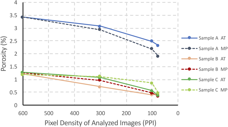 Figure 10. Input image resolution represented by pixel density and porosity (see details in sensitivity test). Solid lines are automatic thresholding (AT) results, whereas dashed lines are manual picking (MP) results. PPI = pixels per inch.
Challenges
Ion-milling SEM is a powerful tool to study mudrock, yet it faces significant challenges. The first is the extremely small area of investigation to provide sufficient resolution, especially under high magnification. Typically, the area of investigation is tens of square micrometers. An upscale from pore-imaging to compositional mapping (e.g., energy dispersive x-ray spectroscopy elemental mapping), then to thin sections scale is an immediate problem. In addition, vertical and lateral heterogeneity in laminated mudrock may vary at the micrometer to centimeter scale (Lazar et al., 2015). To address this issue, large mosaics of SEM images have been used to obtain more representative information about the microstructure of mudrock (Klaver et al., 2012, 2015; Giffin et al., 2013; Hemes et al., 2013, 2015; Houben et al., 2013, 2014; Deirieh, 2016). These studies acquired hundreds of images and stitch them together to cover a large area. Then, a representative elementary area (REA) can be determined, representing the area above which the area fraction of minerals and porosities does not change significantly. However, the REA differs significantly between different samples (Klaver et al., 2012, 2015; Houben et al., 2013, 2014; Hemes et al., 2015; Deirieh, 2016; Kelly et al., 2016). Therefore, it is still very challenging to tell whether an SEM image or a series of images are representative of the mudrock. Last, but not least, even when representativeness is achieved, a significant fraction of the pore system is smaller than the resolution of SEM, especially those pores hosted by OM (Milliken et al., 2013).
Manual Picking versus Automatic Thresholding
To achieve the highest precision when categorizing OM pores and inorganic pores, some scientists prefer manual pore interpretation over automatic pore recognition. As a matter of fact, no absolutely reliable pore segmentation exists; therefore, we have chosen a manually picked result as the reference data sets, although we are aware of the limitation of such a data set. Sometimes, an interpretation of the SEM images is necessary because of artifacts, especially open fractures and redeposition of the milled materials. However, when dealing with a large quantity of images to obtain a statistically REA with a heterogeneous mudrock, manual interpretation can be very time consuming and is subject to operational bias.
The fast development of improved SEM imaging techniques, especially broad ion beam milling, make it urgent to have a consistent methodology of image analysis. The cutting-edge mosaic method and multibeam SEM have begun to address a long-lasting problem in SEM, namely representativeness, by scanning a much bigger area compared with normal SEM. The analysis results are not as strongly affected by the area of investigation and the selection of region of interest. When representativeness is no longer the dominating issue, maintaining the consistency of the results becomes more important. If results are not consistent, one can hardly compare one result with another. Also, the efficiency becomes an issue because of the size of the scanning area and the high resolution, which makes manually processing an image very time consuming.
Effects of Artifacts on Image Analysis
Edge effects are quite common in SEM images of shales. Nonplanar surfaces, such as pore edges, give off a greater electron signal than planar regions, which results in brighter pixels (Kelly et al., 2016). So, these surfaces appear to be a bright “ring” surrounding the OM or minerals (Kelly et al., 2016). This makes it challenging to segment porosity automatically. However, because the edge effect increases the local variance, the segmentation algorithm proposed in this research actually takes advantage of this type of artifact when it occurs.
This method is created based on Zeiss SE2 SEM images. We also tested our workflow on an independently provided image (an FEI BSE SEM image), and the result is shown in Figure 6. The major disagreement between our automatic segmentation and independent third party’s manual picking is marked by the yellow and blue arrows. The method we propose can handle the edge effect very well. But certain very shallow pores exist that are incorrectly labeled as OM because those shallower locations are brighter than deeper pore locations. A similar kind of artifact has also been noticed by Hemes et al. (2013). They referred to this problem as a low-angle deepening pore border, which is marked with yellow arrows in Figure 6B. Canter et al. (2016) argue that the electron beam signal is being reflected from the back of the pore. Disagreements that are marked with blue arrows, unlike other pores or low-angle pore borders, are caused by surface roughness or very shallow dents. For this image, the automated segmented porosity is 2.07%, whereas the manually picked porosity is 3.08%; the pores depicted by blue arrows account for 0.75%. We therefore suggest the correct porosity result should be 2.33%, and our method captured 89% of the whole-pore system. The problematic pores in Figure 6 are all very shallow, so that the detector received signals from the bottom of pores, and, because they are OM-hosted pores, the bottom is obviously OM. The effects and pore back problem seem to be more obvious in the BSE image (Figure 6) than that in SE2 images because the interaction volume of BSE is significantly deeper than SE2. Not to mention, the BSE image was acquired under a higher accelerating voltage (8 kV in this research), which leads to a deeper penetration of the electron beam. Therefore, from a quantitative image analysis point of view, a low beam voltage (1 kV in this research) should be preferred when imaging pores in mudrock reservoirs, especially those OM-hosted pores.
Image Analysis of Organic Matter and Porosity
In this research, most OM in the Mahantango and Marcellus mudrock reservoirs is unstructured. The SEM imaging allows the visualization of the spatial distribution of OM in mudrock. Our data show that the richness of OM in mudrock observed in SEM is correlated with the bulk rock TOC content (Figure 11). The OM content determined by SEM image analysis is much higher than TOC value, which is caused by two main reasons. On the one hand, OM content measures the whole organic materials (kerogen, pyrobitumen, etc.) that are organic compounds with complicated molecular structure. For example, the elemental composition of kerogen from Green River Shale is approximately C215H330O12N5S1 (Robinson, 1976). However, TOC only measures the carbon part. On the other hand, TOC is in weight percentage, whereas OM content measures the area, and it is a proxy for volume percentage. The density of OM is much lower than the rest of the mudrock formation or rock bulk density. Adding the abovementioned two factors together, OM content can be more than three times the value of TOC. Given the representativeness of OM measurements varies (Figure 11), an REA for OM, as well as porosity, needs to be studied, and they are very likely different for a given sample. Although this technique can offer a comprehensive understanding of samples in terms of OM, one should not rely on individual SEM images measurement. Instead, multiple images (10 to 15 in this research) should be acquired.
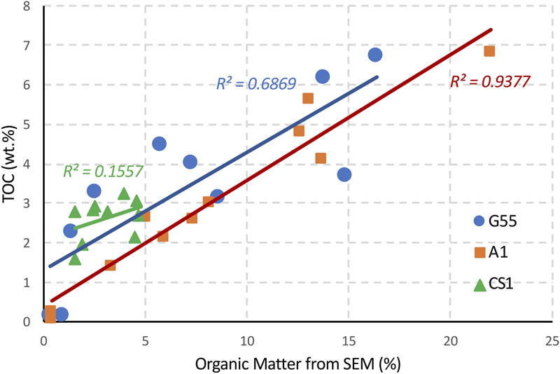 Figure 11. Correlation between organic matter captured by scanning electron microscope (SEM) images and bulk rock total organic carbon (TOC). Notice the x- and y-axis scales are not the same. R2 = coefficient of determination.
The underestimation of porosity remains an issue for SEM, especially 2-D SEM (Loucks et al., 2009; Milliken et al., 2013). The porosity values from SEM images are plotted in Figure 12. Each one of the data points is an average value of 10 to 15 SEM images. Compared with the Gas Research Institute (GRI) method (crushed core analysis), SEM underestimates the porosity (Figure 12), presumably because SEM cannot resolve and detect pores below its resolution of 10 or 15 nm/pixel (in this research), whereas GRI can detect porosity contribution from pores much less than 10 nm (Luffel and Guidry, 1992). The pervasive existence of noise makes it hard to rely on only a few pixels to identify a pore. In this research, we followed McCoy's (2005) suggestion and set the minimum pore size at a three-by-three cluster of pixels. Therefore, the actual minimum pore size analyzed in this research is 30 nm. Milliken et al. (2013) studied samples from the Marcellus Shale and found an unexpected negative correlation between TOC content and SEM visible porosity, although most of the visible pores are hosted by OM (Milliken et al., 2013). Although SEM can achieve a resolution of approximately 1 nm, the area of investigation is reduced to the point at which the observations do not provide an REA. Additionally, 2-D SEM images show slices or cross-sections of samples commonly in the vertical orientation, so 3-D data about the pore space that may be elongated in the third dimension are not measured.
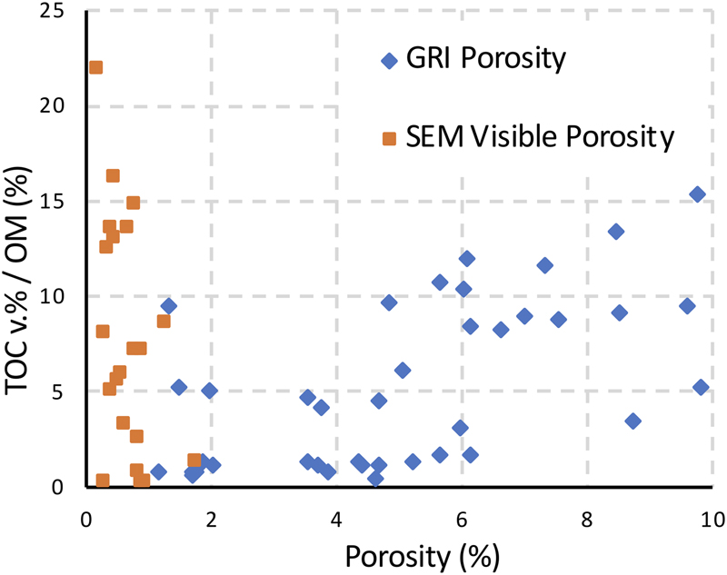 Figure 12. Comparing scanning electron microscope (SEM) visible porosity and Gas Research Institute (GRI) porosity. OM = organic matter; TOC = total organic carbon.
The limitation of SEM should also be taken into consideration. Increasing abundance of OM correlates with decreasing visible porosity in SEM images in the Marcellus Shale (Milliken et al., 2013). When dealing with samples that have a large part of pores below the resolution of SEM, the porosity value from images itself has limited reliability or utility.
CONCLUSION
Ion-milling SEM is a direct analytical technique to facilitate characterizing the microstructure of mudrock reservoir at a resolution of nanometers. Quantitative analysis provides important information regarding pore structure, porosity associated with OM or inorganic minerals, and organic richness. Quantification of SEM images of mudrock samples remains challenging because of the lack of an automated thresholding and segmentation method. Manually picking the threshold is time consuming, and maintaining interlab and intralab consistency is a challenge. Automated segmentation of SEM images using the approach described here offers benefits over manual methods. The key conclusions include the following.
A new workflow is described to quantify porosity and OM content from SEM image analysis. The segmentation of pore space and OM is based on adaptive local thresholding (Phansalkar thresholding), Otsu thresholding, and Image Calculator, all of which can be realized in public domain software such as ImageJ and Fiji. The workflow improves the consistency and efficiency of quantitative image analysis.
The thresholding method segments the image based on local variance. It allows us to take advantage of the very common, yet challenging, edge effect. During the thresholding and segmentation processes, no specific threshold is required, thus avoiding potential bias. The workflow presented here requires minimal supervision, or extra work. However, very shallow depressions require additional work to provide a solution.
The only parameter that needs to be set when running segmentation of pores is the local thresholding window size. Based on our sensitivity test result, for our pore size range, we recommend using 15 pixels for a 600-PPI image, although the result is not very sensitive to the window size (in a range between 10 and 20). The quality of the input image makes bigger contribution to the segmentation result. Lowering the resolution as well as increasing the electron beam voltage will make pores hard to recognize.
Mineral-hosted pores are easier to identify because the contrast between the foreground (pore space) and background (minerals) is larger compared with OM-hosted pores.
This method not only provides the porosity values, but also yields the distribution of pores and OM, a potential input for further research.
This method is created based on Zeiss SE2 SEM images. We also tested it on an FEI BSE SEM image. It successfully captured 89% of the pores when compared with manual segmentation of the BSE image.
7. Quantitative visual analysis of 2-D SE2 SEM images underestimates the porosity compared with the GRI method. This may be the result of differences in pore size resolution between the two radically different methods.
REFERENCES CITED
Ambrose, R. J., R. C. Hartman, M. D. Campos, I. Y. Akkutlu, and C. Sondergeld, 2010, New pore-scale considerations for shale gas in place calculations: Society of Petroleum Engineers Unconventional Gas Conference, Pittsburgh, Pennsylvania, February 23–25, 2010, SPE-131772-MS, 17 p., doi:10.2118/131772-MS.
Anovitz, L. M., and D. R. Cole, 2015, Characterization and analysis of porosity and pore structures: Reviews in Mineralogy and Geochemistry, v. 80, no. 1, p. 61–164, doi:10.2138/rmg.2015.80.04.
Bohacs, K. M., Q. R. Passey, M. Rudnicki, W. L. Esch, and O. R. Lazar, 2013, The spectrum of fine-grained reservoirs from “shale gas” to “shale oil”/tight liquids: Essential attributes, key controls, practical characterization: International Petroleum Technology Conference, Beijing, China, March 26–28, 2013, 16 p., doi:10.2523/16676-MS.
Canter, L., S. Zhang, M. Sonnenfeld, C. Bugge, M. Guisinger, and K. Jones, 2016, Primary and secondary organic matter habit in unconventional reservoirs, in Olson, T., ed., Imaging unconventional reservoir pore systems: AAPG Memoir 112, p. 9–24, doi:10.1306/13592014M1123691.
Culligan, K. A., D. Wildenschild, B. S. B. Christensen, W. G. Gray, and M. L. Rivers, 2006, Pore-scale characteristics of multiphase flow in porous media: A comparison of air–water and oil–water experiments: Advances in Water Resources, v. 29, no. 2, p. 227–238, doi:10.1016/j.advwatres.2005.03.021.
Culligan, K. A., D. Wildenschild, B. S. B. Christensen, W. G. Gray, M. L. Rivers, and A. F. B. Tompson, 2004, Interfacial area measurements for unsaturated flow through a porous medium: Water Resources Research, v. 40, no. 12, 12 p., doi:10.1029/2004WR003278.
Curtis, M. E., R. J. Ambrose, C. H. Sondergeld, and C. S. Rai, 2011, Investigation of the relationship between organic porosity and thermal maturity in the Marcellus Shale: North American Unconventional Gas Conference and Exhibition, The Woodlands, Texas, June 14–16, 2011, 4 p., doi:10.2118/144370-MS.
Curtis, M. E., C. H. Sondergeld, R. J. Ambrose, and C. S. Rai, 2012, Microstructural investigation of gas shales in two and three dimensions using nanometer-scale resolution imaging: AAPG Bulletin, v. 96, no. 4, p. 665–677, doi:10.1306/08151110188.
Deirieh, A., 2016, From clay slurries to mudrocks : A cryo-SEM investigation of the development of the porosity and microstructure: Ph.D. dissertation, Cambridge, Massachusetts, Massachusetts Institute of Technology, 226 p.
Dilks, A., and S. C. Graham, 1985, Quantitative mineralogical characterization of sandstones by back-scattered electron image analysis: Journal of Sedimentary Petrology, v. 55, no. 3, p. 347–355, doi:10.1306/212F86C5-2B24-11D7-8648000102C1865D.
Dong, T., and N. B. Harris, 2013, Pore size distribution and morphology in the horn river shale, Middle and Upper Devonian, northeastern British Columbia, Canada, in W. K Camp, E. Diaz, and B. Wawak, eds., Electron microscopy of shale hydrocarbon reservoirs: AAPG Memoir 102, p. 67–80, doi:10.1306/13391706M1023584.
Driskill, B., J. Walls, J. DeVito, and S. W. Sinclair, 2013, Applications of SEM imaging to reservoir characterization in the Eagle Ford Shale, South Texas, U.S.A., in W. K. Camp, E. Diaz, and B. Wawak, eds., Electron microscopy of shale hydrocarbon reservoirs: AAPG Memoir 102, p. 115–136, doi:10.1306/13391709M1023587.
Erdman, N., and N. Drenzek, 2013, Integrated preparation and imaging techniques for the microstructural and geochemical characterization of shale by scanning electron microscopy, in W. K. Camp, E. Diaz, and B. Wawak, eds., Electron microscopy of shale hydrocarbon reservoirs: AAPG Memoir 102, p. 7–14, doi:10.1306/13391700M1023581.
Espitalie, J., G. Deroo, and F. Marquis, 1985, La pyrolyse Rock-Eval et ses applications. Deuxième partie: Revue de l’Institut Français du Pétrole, v. 40, no. 6, p. 755–784, doi:10.2516/ogst:1985045.
Fishman, N. S., J. L. Ridgley, D. K. Higley, M. L. W. Tuttle, and D. L. Hall, 2012, Ancient microbial gas in the Upper Cretaceous Milk River Formation, Alberta and Saskatchewan: A large continuous accumulation in fine-grained rocks, in Breyer, J. A., ed., Shale reservoirs—Giant resources for the 21st century: AAPG Memoir 97, p. 258–289, doi:10.1306/13321471M973493.
Gallagher, N. C. J., and G. L. Wise, 1981, A theoretical analysis of the properties of median filters: Institute of Electrical and Electronics Engineers Transactions on Acoustics, Speech, and Signal Processing, v. 29, no. 6, p. 1136–1141, doi:10.1109/TASSP.1981.1163708.
Giffin, S., R. Littke, J. Klaver, and J. L. Urai, 2013, Application of BIB–SEM technology to characterize macropore morphology in coal: International Journal of Coal Geology, v. 114, p. 85–95, doi:10.1016/j.coal.2013.02.009.
Hemes, S., G. Desbois, J. L. Urai, M. De Craen, and M. Honty, 2013, Variations in the morphology of porosity in the Boom Clay Formation: Insights from 2D high resolution BIB-SEM imaging and mercury injection porosimetry: Journal of Geosciences, v. 92, no. 4, p. 275–300, doi:10.1017/S0016774600000214.
Hemes, S., G. Desbois, J. L. Urai, B. Schröppel, and J. -O. Schwarz, 2015, Multi-scale characterization of porosity in Boom Clay (HADES-level, Mol, Belgium) using a combination of x-ray μ-CT, 2D BIB-SEM and FIB-SEM tomography: Microporous and Mesoporous Materials, v. 208, p. 1–20, doi:10.1016/j.micromeso.2015.01.022.
Houben, M. E., G. Desbois, and J. L. Urai, 2013, Pore morphology and distribution in the Shaly facies of Opalinus Clay (Mont Terri, Switzerland): Insights from representative 2D BIB-SEM investigations on mm to nm scale: Applied Clay Science, v. 71, p. 82–97, doi:10.1016/j.clay.2012.11.006.
Houben, M. E., G. Desbois, and J. L. Urai, 2014, A comparative study of representative 2D microstructures in shaly and sandy facies of Opalinus Clay (Mont Terri, Switzerland) inferred form BIB-SEM and MIP methods: Marine and Petroleum Geology, v. 49, p. 143–161, doi:10.1016/j.marpetgeo.2013.10.009.
Huang, J., T. Cavanaugh, and B. Nur, 2013, An introduction to SEM operational principles and geologic applications for shale hydrocarbon reservoirs, in W. K. Camp, E. Diaz, and B. Wawak, eds., Electron microscopy of shale hydrocarbon reservoirs: AAPG Memoir 102, p. 1–6, doi:10.1306/13391699M1023580.
Jarvie, D. M., R. J. Hill, T. E. Ruble, and R. M. Pollastro, 2007, Unconventional shale–gas systems: The Mississippian Barnett Shale of north–central Texas as one model for thermogenic shale–gas assessment: AAPG Bulletin, v. 91, no. 4, p. 475–499, doi:10.1306/12190606068.
Javadpour, F., 2009, Nanopores and apparent permeability of gas flow in mudrocks (shales and siltstone): Journal of Canadian Petroleum Technology, v. 48, no. 8, p. 16–21, doi:10.2118/09-08-16-DA.
Katz, A. J., and A. H. Thompson, 1985, Fractal sandstone pores: Implications for conductivity and pore formation: Physical Review Letters, v. 54, no. 12, p. 1325–1328, doi:10.1103/PhysRevLett.54.1325.
Kelly, S., H. El-Sobky, C. Torres-Verdín, and M. T. Balhoff, 2016, Assessing the utility of FIB-SEM images for shale digital rock physics: Advances in Water Resources, v. 95, p. 302–316, doi:10.1016/j.advwatres.2015.06.010.
Klaver, J., G. Desbois, R. Littke, and J. L. Urai, 2015, BIB-SEM characterization of pore space morphology and distribution in postmature to overmature samples from the Haynesville and Bossier Shales: Marine and Petroleum Geology, v. 59, p. 451–466, doi:10.1016/j.marpetgeo.2014.09.020.
Klaver, J., G. Desbois, J. L. Urai, and R. Littke, 2012, BIB-SEM study of the pore space morphology in early mature Posidonia Shale from the Hils area, Germany: International Journal of Coal Geology, v. 103, p. 12–25, doi:10.1016/j.coal.2012.06.012.
Lazar, O. R., K. M. Bohacs, J. H. S. Macquaker, J. Schieber, and T. M. Demko, 2015, Capturing key attributes of fine-grained sedimentary rocks in outcrops, cores, and thin sections: Nomenclature and description guidelines: Journal of Sedimentary Research, v. 85, no. 3, p. 230–246, doi:10.2110/jsr.2015.11.
Loucks, R. G., R. M. Reed, S. C. Ruppel, and U. Hammes, 2012, Spectrum of pore types and networks in mudrocks and a descriptive classification for matrix-related mudrock pores: AAPG Bulletin, v. 96, no. 6, p. 1071–1098, doi:10.1306/08171111061.
Loucks, R. G., R. M. Reed, S. C. Ruppel, and D. M. Jarvie, 2009, Morphology, genesis, and distribution of nanometer-scale pores in siliceous mudstones of the Mississippian Barnett Shale: Journal of Sedimentary Research, v. 79, no. 12, p. 848–861, doi:10.2110/jsr.2009.092.
Luffel, D. L., and F. K. Guidry, 1992, New core analysis methods for measuring reservoir rock properties of Devonian Shale: Journal of Petroleum Technology, v. 44, no. 11, p. 1184–1190, doi:10.2118/20571-PA.
McCoy, R. M., 2005, Field methods in remote sensing: New York, The Guilford Press, 159 p.
Milliken, K. L., R. J. Day-Stirrat, P. K. Papazis, and C. Dohse, 2012, Carbonate lithologies of the Mississippian Barnett Shale, Fort Worth Basin, Texas, in J. A. Breyer, ed., Shale reservoirs—Giant resources for the 21st century: AAPG Memoir 97, p. 290–321, doi:10.1306/13321473M97252.
Milliken, K. L., L. T. Ko, M. Pommer, and K. M. Marsaglia, 2014, Sem petrography of eastern Mediterranean Sapropels: Analogue data for assessing organic matter in oil and gas shales: Journal of Sedimentary Research, v. 84, no. 11, p. 961–974, doi:10.2110/jsr.2014.75.
Milliken, K. L., and T. Olson, 2016, Amorphous and crystalline solids as artifacts in SEM images, in T. Olson, ed., Imaging unconventional reservoir pore systems: AAPG Memoir 112, p. 1–8, doi:10.1306/13592013M112252.
Milliken, K. L., M. Rudnicki, D. N. Awwiller, and T. Zhang, 2013, Organic matter–hosted pore system, Marcellus Formation (Devonian), Pennsylvania: AAPG Bulletin, v. 97, no. 2, p. 177–200, doi:10.1306/07231212048.
Nole, M., H. Daigle, K. L. Milliken, and M. Prodanović, 2016, A method for estimating microporosity of fine-grained sediments and sedimentary rocks via scanning electron microscope image analysis: Sedimentology, v. 63, no. 6, p. 1507–1521, doi:10.1111/sed.12271.
Otsu, N., 1979, A threshold selection method from gray-level histograms: IEEE Transactions on Systems, Man, and Cybernetics, v. 9, no. 1, p. 62–66, doi:10.1109/TSMC.1979.4310076.
Passey, Q. R., K. M. Bohacs, W. L. Esch, R. E. Klimentidis, and S. K. Sinha, 2012, My source rock is now my reservoir - Geologic and petrophysical characterization of shale-gas reservoirs (abs.): The Society for Organic Petrology 28th Annual Meeting, Halifax, Nova Scotia, Canada, July 31–August 4, 2011, accessed June 25, 2012, http://archives.datapages.com/data/tsop/TSOPv28_2011/passey.htm.
Phansalkar, N., S. More, A. Sabale, and M. Joshi, 2011, Adaptive local thresholding for detection of nuclei in diversity stained cytology images: International Conference on Communications and Signal Processing, Calicut, India, February 10–12, 2011, p. 218–220.
Pommer, M., and K. Milliken, 2015, Pore types and pore-size distributions across thermal maturity, Eagle Ford Formation, southern Texas: AAPG Bulletin, v. 99, no. 9, p. 1713–1744, doi:10.1306/03051514151.
Robinson, W. E., 1976, Origin and characteristics of green river oil shale, in T. F. Yen and G. V. Chilingarian, eds., Oil shale: Developments in Petroleum Science, v. 5, p. 61–79, doi:10.1016/S0376-7361(08)70044-X.
Ross, D. J. K., and R. M. Bustin, 2009, The importance of shale composition and pore structure upon gas storage potential of shale gas reservoirs: Marine and Petroleum Geology, v. 26, no. 6, p. 916–927, doi:10.1016/j.marpetgeo.2008.06.004.
Saidian, M., U. Kuila, M. Prasad, L. Alcantar Lopez, S. Riveral, and L. J. Godinez, 2015, A comparison of measurement techniques for porosity and pore size distribution in shales (mudrocks): A case study of Haynesville, Niobrara, Monterey and Eastern European Silurian Formations, in Olson, T., ed., Imaging unconventional reservoir pore systems: AAPG Memoir 112, p. 89–114, doi:10.1306/13592019M1123695.
Sauvola, J., and M. Pietikainen, 2000, Adaptive document image binarization: Pattern Recognition, v. 33, no. 2, p. 225–236, doi:10.1016/S0031-3203(99)00055-2.
Schieber, J., 2010, Common themes in the formation and preservation of intrinsic porosity in shales and mudstones Illustrated with examples across the Phanerozoic: Society of Petroleum Engineers Unconventional Gas Conference, Pittsburgh, Pennsylvania, February 23–25, 2010, 10 p., doi:10.2118/132370-MS.
Schieber, J., 2013, SEM observations on ion-milled samples of Devonian black shales from Indiana and New York: The petrographic context of multiple pore types, in W. K. Camp, E. Diaz, and B. Wawak, eds., Electron microscopy of shale hydrocarbon reservoirs: AAPG Memoir 102, p. 153–172, doi:10.1306/13391711M1023589.
Schieber, J., R. Lazar, K. Bohacs, R. Klimentidis, M. Dumitrescu, and J. Ottmann, 2016, An SEM study of porosity in the Eagle Ford shale of Texas—Pore types and porosity distribution in a depositional and sequence-stratigraphic context: AAPG Memoir 110, p. 167–186, doi:10.1306/13541961M1103589.
Schindelin, J., I. Arganda-Carreras, E. Frise, V. Kaynig, M. Longair, T. Pietzsch, and S. Preibisch, et al., 2012, Fiji: An open source platform for biological-image analysis: Nature Methods, v. 9, no. 7, p. 676–682, doi:10.1038/nmeth.2019.
Schindelin, J., C. T. Rueden, M. C. Hiner, and K. W. Eliceiri, 2015, The ImageJ ecosystem: An open platform for biomedical image analysis: Molecular Reproduction and Development, v. 82, no. 7–8, p. 518–529, doi:10.1002/mrd.22489.
Schneider, C., W. S. Rasband, and K. W. Eliceiri, 2012, NIH Image to ImageJ: 25 years of image analysis: Nature Methods, v. 9, no. 7, p. 671–675, doi:10.1038/nmeth.2089.
Sezgin, M., and B. Sankur, 2004, Survey over image thresholding techniques and quatitative performance evaluation: Journal of Electronic Imaging, v. 13, no. 1, p. 146–168, doi:10.1117/1.1631315.
Slatt, R. M., and N. R. O’Brien, 2011, Pore types in the Barnett and Woodford gas shales: Contribution to understanding gas storage and migration pathways in fine-grained rocks: AAPG Bulletin, v. 95, no. 12, p. 2017–2030, doi:10.1306/03301110145.
Slatt, R. M., and N. R. O’Brien, 2013, Microfabrics related to porosity development, sedimentary and diagenetic processes, and composition of unconventional resource shale reservoirs as determined by conventional scanning electron microscopy, in W. K. Camp, E. Diaz, and B. Wawak, eds.,Electron microscopy of shale hydrocarbon reservoirs: AAPG Memoir 102, p. 37–44, doi:10.1306/13391703M102441.
Sondergeld, C. H., R. J. Ambrose, C. S. Rai, and J. Moncrieff, 2010a, Micro-structural studies of gas shales: Society of Petroleum Engineers Unconventional Gas Conference, Pittsburgh, Pennsylvania, February 23–25, 2010, SPE-131771-MS, 17 p., doi:10.2118/131771-MS.
Sondergeld, C. H., K. E. Newsham, J. T. Comisky, M. C. Rice, and C. S. Rai, 2010b, Petrophysical considerations in evaluating and producing shale gas resources: Society of Petroleum Engineers Unconventional Gas Conference, Pittsburgh, Pennsylvania, February 23–25, 2010, SPE-131768-MS, 34 p., doi:10.2118/131768-MS.
US Energy Information Administration, 2017, Annual energy outlook: Washington, DC, US Energy Information Administration, 64 p.
Walls, J. D., and S. W. Sinclair, 2011, Eagle Ford shale reservoir properties from digital rock physics: First Break, v. 29, no. 6, p. 97–101.
Wildenschild, D., and A. P. Sheppard, 2013, X-ray imaging and analysis techniques for quantifying pore-scale structure and processes in subsurface porous medium systems: Advances in Water Resources, v. 51, p. 217–246, doi:10.1016/j.advwatres.2012.07.018.
Zagorski, W. A., G. R. Wrightstone, and D. C. Bowman, 2012, The Appalachian Basin Marcellus gas play: Its history of development, geologic controls on production, and future potential as a world-class reservoir, in Breyer, J. A., ed., Shale reservoirs—Giant resources for the 21st century: AAPG Memoir 97, p. 172–200, doi:10.1306/13321465M973491.
Zhang, H., J. E. Fritts, and S. A. Goldman, 2008, Image segmentation evaluation: A survey of unsupervised methods: Computer Vision and Image Understanding, v. 110, no. 2, p. 260–280, doi:10.1016/j.cviu.2007.08.003.
Zhang, S., R. E. Klimentidis, and P. Barthelemy, 2011, Porosity and permeability analysis on nanoscale FIB-SEM 3D imaging of shale rock: International Symposium of the Society of Core Analysts, Austin, Texas, September 18–21, 2011, 12 p.
ACKNOWLEDGMENTS
The research undertaken in this study was funded through the US Department of Energy (DOE) National Energy Technology Laboratory as part of their Marcellus Shale Energy and Environmental Laboratory (DOE Award DE-FE0024297). We thank the Energy Corporation of America and the Petroleum Development Corporation for providing the cores and Ingrain for providing high-quality scanning electron microscope images. Fiji and ImageJ software developed by National Institutes of Health are used in this project. We also thank our reviewers, especially Terrilyn Olson and AAPG Editor Barry J. Katz, whose constructive input and guidance greatly improved the manuscript.
DATASHARE 107
Step-by-Step ImageJ/Fiji Procedure is available in an electronic version on the AAPG website (www.aapg.org/datashare) as Datashare 107.