ABSTRACT
Petroleum companies have invested heavily in the exploration of frontier offshore basins in Brazil. Uncertainties associated with geologic complexity, lithostratigraphy, fluid content, and seismic resolution in these basins are the most common challenges. Many methods have been used to circumvent these issues, such as assessing seismic attributes, seismic inversion, spectral decomposition, and the integration of these methodologies to accomplish an optimal approach. Because of the complex geology of these areas, it is very difficult to identify potential reservoirs within one specific geologic formation. Hence, applying spectral decomposition to frontier basins of high geologic complexity can help overcome the challenges because in the frequency domain, it is possible to better define variability and lateral discontinuities. The correct choice of the spectral decomposition optimization approach is critical for accurate target zone representation as well as selection of the appropriate transform. Prestack inversion, spectral decomposition, and attribute seismic facies classification were applied to evaluate the extent of a reservoir and analyze whether an appraisal well has been sited at a good location. The results showed that the new appraisal well was planned at a good location but that its facies were not as good as those of the first discovery well, as confirmed after drilling.
INTRODUCTION
The aim of this paper is to present a workflow to reduce exploration risk through the integration of seismic attributes, including spectral decomposition, prestack inversion, and seismic facies classification, thus determining the extent of a reservoir, characterizing it, and analyzing whether a second well had been planned at a good location. The methodology was applied to a frontier Brazilian basin, which is an offshore deep- and ultradeep-water zone where the main targets are located in the rift and sag sequences. An exploratory well in this zone revealed oil with reasonable API gravity values ranging from 23° to 27°, with the main reservoir deposited during the sag basin phase.
Spectral decomposition transforms temporal signals into energy density maps. Many methods are available to express the energy of the signal as a function of frequency and amplitude. Each method has its advantages and disadvantages, and different applications require different transforms and specific optimization (Castagna and Sun, 2006). Spectral decomposition has been successfully applied in seismic exploration for stratigraphic mapping (Partyka et al., 1999; Marfurt and Kirlin, 2001; Puryear and Castagna, 2008), reservoir detection (Castagna et al., 2003; Sinha et al., 2005), and attenuation estimation and correction (Lupinacci and Oliveira, 2015), therefore helping to decrease uncertainties encountered during the exploration and production phases and assisting the identification of the best regions for drilling new wells (Jesus et al., 2019).
To define the best spectral decomposition approach to be used, the application, quality of seismic illumination, frequency range, signal-noise ratio, and geologic complexity must be taken into account. A good practice is to conduct a feasibility study to establish the most appropriate spectral decomposition method depending on the purpose of its use. In addition, horizon mapping of an extensive seismic survey may result in many errors because of autopicking, with complex geology limiting the use of horizon slices for spectral decomposition optimization because they cannot represent a geologic timeline. Integration of different seismic attributes, such as compressional (P) and shear (S) impedances as well as the compressional velocity and shear velocity (Vp/Vs) ratio, can help overcome these problems.
Prestack seismic inversion has been applied as a tool for the quantitative seismic interpretation, helping to characterize reservoirs (see, e.g., Avseth et al., 2005; Zhao et al., 2017). The elastic parameters (P- and S-impedances and Vp/Vs ratio) obtained from seismic inversion are correlated with rock physical models, providing information about lithology, fluid content, and porosity (Spikes et al., 2007; Simm and Bacon, 2014). From the seismic inversion and rock physics modeling, static models of reservoir properties are built and thus can assist in reserves estimation (Vernik et al., 2002) as well as estimation of the location of production and injection wells; they can also be used as inputs for flow simulations in dynamic models (Bredesen et al., 2015; Ferreira and Lupinacci, 2018).
Dominant frequency and maximum negative amplitude are other useful seismic attributes that can contribute to optimization of spectral decomposition. When aiming to analyze the dominant frequency in a target zone interval, it is very important to establish which frequencies best represent the potential reservoir. In addition, the maximum negative amplitude between the top and base of the reservoir should be analyzed to assist in the determination of best areas for production because its response is mostly connected to hydrocarbon anomalies or good-quality reservoirs (Jesus et al., 2019).
Finally, seismic facies classification through unsupervised neural network methods is a very powerful tool for reservoir characterization because it allows fast data analysis through the identification of linear or nonlinear correlations among the input seismic attribute volumes and generates facies expected for the area, helping to identify the best reservoir facies when associated to well information (Deboeck and Kohonen, 1998; Du and Swamy, 2014; Shanmuganathan, 2016; Ferreira et al., 2019).
METHODOLOGY
Seismic Data Acquisition and Processing
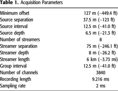
The acquisition parameters are shown in Table 1. The streamer length was approximately 6 km (∼3.73 mi) in an environment with huge submarine canyons and cliffs with bathymetric variation of up to approximately 400 m (∼1300 ft) (Figure 1). Such an acquisition survey might compromise the rays, resulting in target zone poor illumination. Poor illumination was also observed at the greatest depths because of natural energy absorption and a low contribution from the far-offset data because of the short cable length.
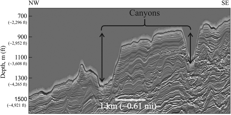 Figure 1. Submarine canyons showing the complex bathymetry of the study area, which impact the seismic imaging of the reservoir zone.
To obtain better images from the subsurface, the seismic data were processed using a specific workflow. The complete flowchart is presented in Figure 2. The complete seismic processing history is not described in this paper. However, two main steps that were used to achieve considerable analytical improvements are highlighted: water column statics (WCS) correction and velocity model building (VMB). The WCS correction was applied to compensate for velocity changes in the water column caused by salinity, temperature, and density. As for VBM, the initial step applied was a tomographic model. Then, a tilted transversal isotropic model was obtained from the tomographic approach, along with three seismic and well data inversions (Bakulin et al., 2010). To decrease the well-to-seismic misties, the anisotropy models were updated based on well markers.
 Figure 2. Seismic processing workflow applied for improved seismic imaging. 3-D = three-dimensional.
An important strategy was adopted in the data processing to prevent the velocity model from following sea-floor variation or creating “bull eyes” in the final model, which consisted of building the velocity model starting with the low frequencies and then refining it by adding the higher frequencies in each round of tomography. Occasionally, the tomographic signal was lost, converging to a local minimum because of poor illumination associated with the highly complex sea-floor topography.
Seismic Data Preconditioning
Seismic data usually contain random and coherent noise. This noise may be caused by acquisition design, preprocessing, and migration (Chopra and Marfurt, 2007). Nevertheless, some of those problems can be mitigated through poststack processing before generating seismic attributes.
The seismic migration data were preconditioned through two stages, each having different objectives. First, a structurally oriented filtering was applied to improve the signal-noise ratio, which can make the seismic reflector more continuous, and better define faults. Then, spectral enhancement was used to improve vertical resolution (Zhou et al., 2014). As shown in Figure 3, these steps preserved the original dominant frequency and accentuated the preexisting frequencies, thereby increasing bandwidth and improving the vertical resolution.
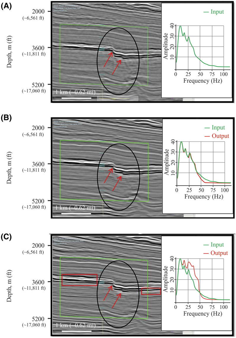 Figure 3. (A) Original seismic section. (B) Seismic section after application of the structurally oriented filtering. (C) Seismic section after application of the spectral enhancement. It is possible to notice the increase of the seismic resolution after preconditioning and better definition of layers as shown in the red boxes.
Prestack Inversion
Information obtained from prestack inversion may facilitate the identification of facies within the target zone. The use of elastic attributes to optimize spectral decomposition can increase the reliability for identification of lithology and fluid type (Jesus and Takayama, 2016). In this study, prestack inversion was used to discriminate sands from shales, and spectral decomposition was performed, only considering the dominant frequency value corresponding to the sand zones.
When elastic attributes, such as Vp and Vs, acoustic impedance (Ip), and density, are known, predictions of petrophysical parameters, characterization of rock heterogeneity and complexity, as well as their uncertainty associated with theoretical modeling are the main objectives of rock physics inversion (Grana and Della Rossa, 2010). A combination of rock physics inversion and seismic inversion facilitates estimation of petrophysical properties (Grana, 2016), and when petrophysical properties and their uncertainties can be estimated, it is possible to assess the probable facies occurrence (Xu et al., 2016).
Seismic inversion attributes (Ip and Vp/Vs) and lithological information from the wells were used to obtain facies and fluid probabilities (FFP) through Bayesian inference (Pendrel et al., 2017; Schwedersky et al., 2017). The FFP helped in the uncertainty analysis for reservoir evaluation. Three volumes resulting from FFP analysis based on the construction of probability density functions on an Ip and Vp/Vs crossplot were generated: good-quality sandstone reservoir, poor-quality sandstone reservoir, and shale.
Spectral Decomposition
Conventional spectral decomposition methodologies consider horizon slices or time slices to optimize their results. However, geologic complexity inhibits the accuracy of these conventional approaches. Focusing solely on the reservoir area, elastic inversion attributes were used to optimize spectral decomposition and increase the reliability of results, assisting in the interpretations (Veeken and Da Silva, 2004). Then, a sensitivity study was performed using the top and base of the interpreted horizons from the elastic inversion result, as well as the seismic volume following structurally oriented filtering and spectral enhancement, to calculate the maximum negative amplitude and dominant frequency. With the maximum negative amplitude and dominant frequency attributes (Figure 4), both the discovery well and the first appraisal well locations were evaluated. Based on the maximum negative amplitude map, both wells are in a strong negative amplitude zone, but the signal is weaker for the appraisal well.
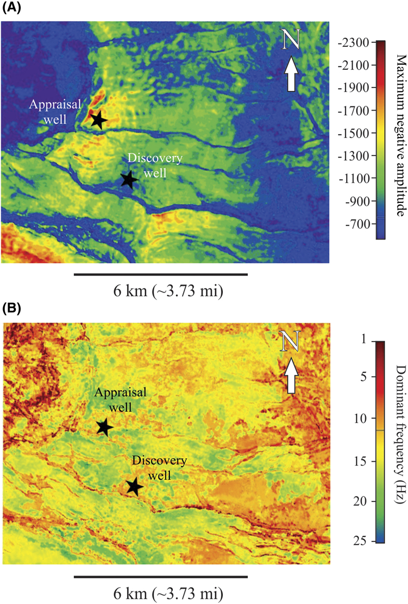 Figure 4. (A) Maximum negative amplitude and (B) dominant frequency (hertz) extracted between the top and base of the reservoir.
Spectral decomposition basically decomposes the seismic data into different frequency bands, as illustrated in Figure 5. The seismic data in the time domain were used for spectral decomposition because the algorithm assesses spectral components in the time-frequency domain (measured in cycles per second or hertz). However, the results are later converted to the depth domain using the existing VMB for enhanced accuracy and to have more control over tuning effects.
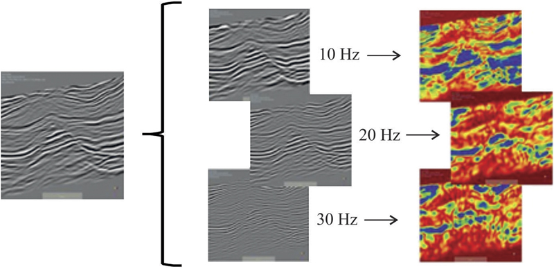 Figure 5. Short-time window Fourier transform was applied to seismic data, decomposing it into frequency bands; then, envelope attributes were calculated for each frequency band.
Based on the analysis of dominant frequency, the reservoir exhibits mainly a low frequency of 10 Hz. Also, the base of the reservoir has a strong negative amplitude, and the most important frequencies in the reservoir were identified through a sensitivity study that indicated frequency bands of 10, 20, and 30 Hz, which were used for analysis. Then, the envelope attribute, which contained amplitude information for each specific range, was calculated for each of the selected frequency bands (Figure 6).
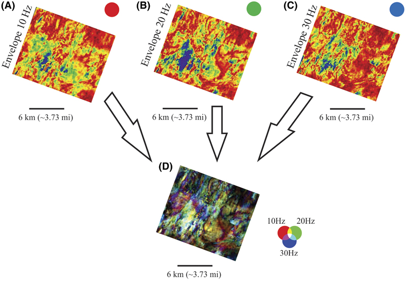 Figure 6. Envelope attributes: (A) red for low frequency (10 Hz), (B) green for mid frequency (20 Hz), and (C) blue for high frequency (30 Hz), showing how the red, green, and blue blend (D) was created.
Spectral decomposition using short-time window Fourier transform (SWFT) was applied to the seismic volume following preconditioning and spectral enhancement. The SWFT spectral decomposition uses a time window, which influences the frequency as well as temporal and spatial resolutions. Narrower windows provide good vertical resolution but generate low-frequency resolution (Addison, 2002). The main objective of using SWFT is to obtain high-frequency resolution to better understand the spatial distribution of seismic facies while balancing this with an acceptable vertical resolution. Therefore, SWFT was applied with a time window of 30 ms based on seismic data from well logs and markers. According to Chopra and Marfurt (2014), the window width should be carefully chosen because analysis of windows that are smaller than the period of interest can create Gibbs artifacts.
Seismic Facies Classification
An unsupervised neural network was used for seismic facies classification based on the self-organizing maps method defined by Kohonen (1990, 2013). The application of this method is based entirely on the characteristics of seismic data, and the resulting facies are indicative of reservoir heterogeneity (Jesus et al., 2019).
The combination of different seismic attributes increases analytical complexity for seismic facies classification. Principal component analysis (PCA) can be used to assess a large set of seismic attributes (Chopra and Marfurt, 2014) and also helps to reveal the most significant seismic attributes (Roden et al., 2015), thereby minimizing redundancy. To perform a PCA, the spectral decomposition, coherence, Ip, and dominant frequency attributes were selected to reveal distribution patterns in the reservoir. Coherence is a measure of similarity between waveforms or traces (Chopra and Marfurt, 2007). This geometrical attribute is helpful to identify faults and fractures, which are important features at the margins of a basin. In addition, Ip can be an excellent tool to estimate the petrophysical parameters of a reservoir (Sancevero et al., 2006), and low-frequency seismic anomalies may be associated with reservoirs (Castagna et al., 2003). The first three resulting principal component vectors were used as inputs for seismic facies classification. As for the unsupervised neural network parametrization, 5 classes were selected for data discrimination in 60 iterations.
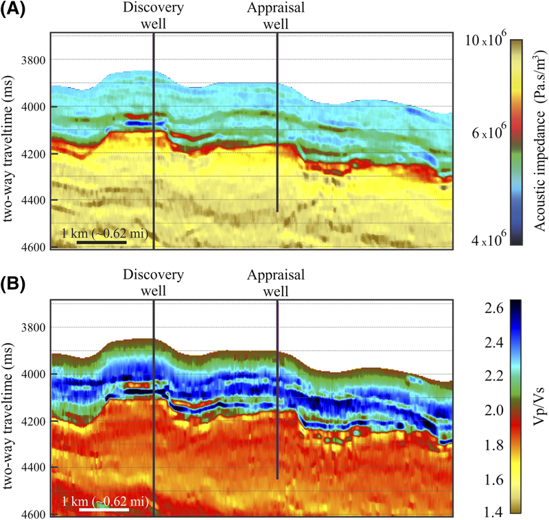 Figure 7. Section view of an arbitrary line crossing discovery and appraisal wells of (A) acoustic impedance values and (B) compressional velocity and shear velocity (Vp/Vs) ratio values.
RESULTS
The Ip and Vp/Vs ratio obtained from prestack inversion are shown in Figure 7A, B, respectively. Using the Ip, Vp/Vs ratio, and clay volume discovery well logs crossplot (Figure 8A), it was possible to identify the sandstones that may contain oil (termed “good-quality sandstones”), identifiable by intermediate Ip and low Vp/Vs ratio values. Shales were characterized by low Ip and high Vp/Vs ratio values. The sandstones with lower probability of oil (termed “poor-quality sandstones”) were classified as the rest of the points in the crossplot with high Ip values and intermediate Vp/Vs ratio values. The regions of good-quality sandstones and shales in the Ip volume, using the limits established by the crossplot analysis, are highlighted in Figure 8B, C, respectively. As can be seen in Figure 8B, both wells are good-quality sandstone locations. The seismic inversion attributes aided in top and bottom mapping and also in optimizing the spectral decomposition and limiting propagation of uncertainty in subsequent steps.
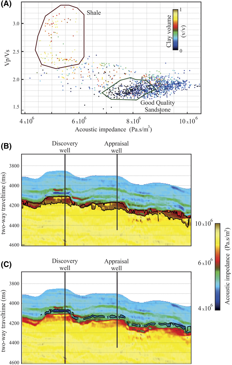 Figure 8. (A) Crossplot between the acoustic impedance and compressional velocity and shear velocity (Vp/Vs) ratio discovery well logs colored by the clay volume log, with polygons highlighting the good-quality sandstones and shales. (B) Section view of an arbitrary line in the seismic impedance volume in which the good-quality sandstones are highlighted according to the crossplot. (C) Section view of an arbitrary line in the seismic impedance volume in which the shales are highlighted according to the crossplot.
Figure 9A–C shows probabilities of each facies in a section, and Figure 9D shows the most probable facies, revealing three different facies identified as shales at the top of the section, shales immediately below the good-quality sandstones, and the poor-quality sandstones at the bottom of the section. It is important to highlight that the actual facies of the discovery well show good correlation with the estimated facies.
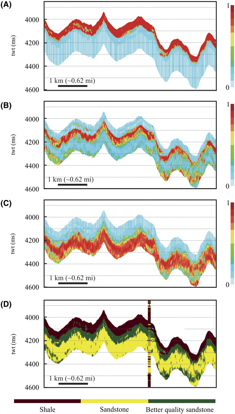 Figure 9. Sections with (A) probabilities of good-quality sandstones, (B) probabilities of shales, (C) probabilities of poor-quality sandstones, and (D) most probable facies compared with the facies log from the discovery well. twt = two-way traveltime.
As for the spectral decomposition results, envelope attributes were calculated for each one of the selected frequencies, and a red, green, and blue (RGB) blend was created: red for low frequency (10 Hz), green for intermediate frequency (20 Hz), and blue for high frequency (30 Hz). The spectral decomposition RGB blends were compared in time and depth domains as a quality control to verify if both results were consistent (Figure 10).
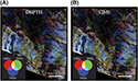 Figure 10. Quality control comparison of spectral decomposition red, green, and blue blends in the depth (A) and time (B) domains from a horizon slice.
These spectral decomposition RGB blends are a mix of three attributes, and the differences in frequencies and magnitude are associated with primary colors. Color variation represents frequency changes, whereas brightness represents changes in amplitude (strong brightness can mean strong positive or negative amplitudes).
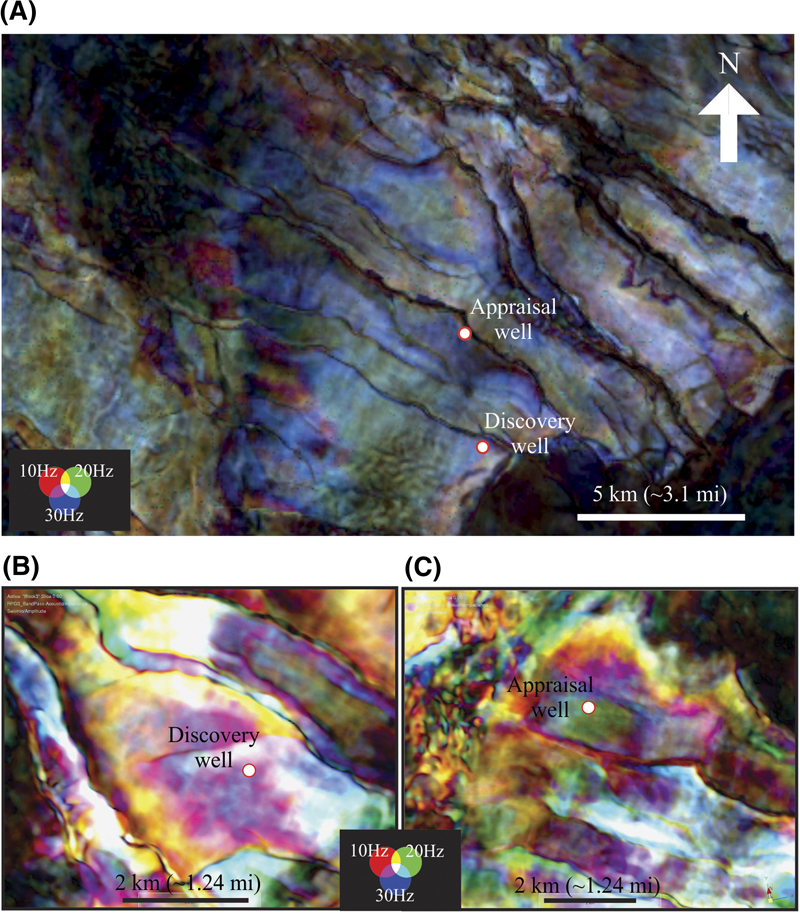 Figure 11. Enhanced view of the spectral decomposition red, green, and blue blend for (A) both the discovery and appraisal wells in the study area, (B) zooming in the discovery well, and (C) magnified view of appraisal well.
The spectral decomposition RGB blends revealed that the profile at the discovery well is quite different from the appraisal well location. According to elastic inversion interpretations, the appraisal well would be a good place to find good-quality sandstones because it has the same characteristics as the discovery well location, but the spectral decomposition RGB blends suggest otherwise because they indicate differences between the two well locations (Figure 11A). The region at the discovery well is brighter and has a purple color, resulting from a mixture of 10- and 30-Hz frequencies, interpreted to be indicative of cleaner sandstones (Figure 11B). As for the region at the appraisal well, a more opaque green color can be seen, resulting from dominance of the 20-Hz frequency, which could indicate shalier sandstone facies in the appraisal well (Figure 11C). Therefore, the results from spectral decomposition analysis indicate that the appraisal well location had a high probability for finding nonreservoir facies. The seismic facies classification results can be observed in an arbitrary line through the two wells in Figure 12 and compared to well data in Figure 13A, B. Porosity and gamma-ray logs were used to qualitatively interpret each class, and because the higher porosity and lower gamma-ray (related to shale content) values indicate the best reservoir classes, the analyzed interval was divided into the following: (1) very good reservoir, (2) good, (3) moderate, (4) poor, and (5) very poor.
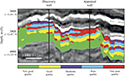 Figure 12. Section view of an arbitrary line crossing the discovery and appraisal wells of seismic facies classification results.
DISCUSSION
Predictions about the appraisal well in the seismic facies classification process were performed using only information from the discovery well. The discovery well is in a better location than the proposed appraisal well because the upper layer in the appraisal well is categorized as very poor quality compared with the discovery well. These results are consistent with the spectral decomposition results.
 Figure 13. Gamma-ray and total porosity logs versus seismic facies classification at the discovery well (A) and appraisal well (B) locations. GAPI = API gravity.
After drilling the appraisal well, its porosity and gamma-ray logs (Figure 13B) were also compared with the seismic facies classification results. This comparison confirmed that the seismic classification and spectral decomposition analysis were accurate because well-log information from the appraisal well revealed the upper part of the well to be shalier, hence possessing poorer-quality reservoirs compared with the discovery well.
CONCLUSION
The preconditioning of seismic data and optimization approach used were critical to guaranteeing that the target zone was accurately represented in the spectral decomposition method. Elastic inversion results indicated that the discovery and appraisal well locations had good-quality sandstones as reservoir facies. However, the spectral decomposition analysis indicated otherwise because it showed different signals at the well locations. These differences were interpreted as an indication of cleaner sandstones at the discovery well and shalier sandstones at the appraisal well. Seismic facies classification was achieved using a combination of acoustic inversion, coherence, dominant frequency, and spectral decomposition attributes, resulting in a satisfactory outcome and exhibiting a good correlation with porosity and gamma-ray well-log data. Again, these results showed that the appraisal well had a poorer reservoir quality when compared with the discovery well, as predicted by the spectral decomposition. The proposed methodology would have allowed the prediction of reservoir potential before the appraisal well was drilled, which was confirmed by drilling, thus proving the effectiveness of the proposed approach in reducing exploration risk.
REFERENCES CITED
Addison, P. S., 2002, The illustrated wavelet transform handbook: Introductory theory and applications in science, engineering, medicine and finance: Boca Raton, Florida, CRC Press, 368 p.
Avseth, P., T. Mukerji, and G. Mavko, 2005, Quantitative seismic interpretation, applying rock physics to reduce interpretation risk: Cambridge, United Kingdom, Cambridge University Press, 376 p.
Bakulin, A., M. Woodward, D. Nichols, K. Osypov, and O. Zdraveva, 2010, Building tilted transversely isotropic depth models using localized anisotropic tomography with well information: Geophysics, v. 75, no. 4, p. D27–D36, doi:10.1190/1.3453416.
Bredesen, K., E. H. Jensen, T. A. Johansen, and P. Avseth, 2015, Quantitative seismic interpretation using inverse rock physics modelling: Petroleum Geoscience, v. 21, no. 4, p. 271–284, doi:10.1144/petgeo2015-006.
Castagna, J., and S. Sun, 2006, Comparison of spectral decomposition methods: First Break, v. 24, no. 3, p. 75–79.
Castagna, J. P., S. Sun, and R. W. Siegfried, 2003, Instantaneous spectral analysis: Detection of low-frequency shadows associated with hydrocarbons: Leading Edge, v. 22, no. 2, p. 120–127, doi:10.1190/1.1559038.
Chopra, S., and K. J. Marfurt, 2007, Structure-oriented filtering and image enhancement, in Seismic attributes for prospect identification and reservoir characterization: Tulsa, Oklahoma, Society of Exploration Geophysicists and European Association of Geoscientists and Engineers, Geophysical Developments Series, p. 187–218.
Chopra, S., and K. J. Marfurt, 2014, Churning seismic attributes with principal component analysis: Society of Exploration Geophysicists International Exposition and Annual Meeting, Denver, Colorado, October 26–31, 2014, p. 2672–2676, doi:10.1190/segam2014-0235.1.
Deboeck, G., and T. Kohonen, eds., 1998, Visual explorations in finance: London, Springer Finance, 229 p.
Du, K., and M. N. S. Swamy, 2014, Neural networks and statistical learning: London, Springer, 824 p.
Ferreira, D. J. A., and W. M. Lupinacci, 2018, An approach for three-dimensional quantitative carbonate reservoir characterization in the Pampo field, Campos Basin, offshore Brazil: AAPG Bulletin, v. 102, no. 11, p. 2267–2282, doi:10.1306/04121817352.
Ferreira, D. J. A., W. M. Lupinacci, I. A. Neves, J. P. R. Zambrini, A. L. Ferrari, L. A. P. Gamboa, and M. Olho Azul, 2019, Unsupervised seismic facies classification applied to a presalt carbonate reservoir, Santos Basin, offshore Brazil: AAPG Bulletin, v. 103, no. 4, p. 997–1012, doi:10.1306/10261818055.
Grana, D., 2016, Rock physics modeling in conventional reservoirs, in C. Jin and G. Cusatis, eds., New frontiers in oil and gas exploration: Cham, Switzerland, Springer International Publishing, p. 137–163, doi:10.1007/978-3-319-40124-9_4.
Grana, D., and E. Della Rossa, 2010, Probabilistic petrophysical-properties estimation integrating statistical rock physics with seismic inversion: Geophysics, v. 75, no. 3, p. O21–O37, doi:10.1190/1.3386676.
Jesus, C., M. Olho Azul, W. M. Lupinacci, and L. Machado, 2019, Multiattribute framework analysis for the identification of carbonate mounds in the Brazilian presalt zone: Interpretation, v. 7, no. 2, p. 1–10, doi:10.1190/INT-2018-0004.1.
Jesus, C., and P. Takayama, 2016, Reducing exploration risk with spectral decomposition: Rio Oil and Gas 2016 Expo and Conference, Rio de Janeiro, Brazil, October 24–27, 2016, 5 p.
Kohonen, T., 1990, The self-organizing map: Proceedings of the IEEE, v. 78, no. 9, p. 1464–1480, doi:10.1109/5.58325.
Kohonen, T., 2013, Essentials of the self-organizing map: Neural Networks, v. 37, p. 52–65, doi:10.1016/j.neunet.2012.09.018.
Lupinacci, W. M., and S. A. M. Oliveira, 2015, Q factor estimation from the amplitude spectrum of the time–frequency transform of stacked reflection seismic data: Journal of Applied Geophysics, v. 114, p. 202–209, doi:10.1016/j.jappgeo.2015.01.019.
Marfurt, K. J., and R. L. Kirlin, 2001, Narrow‐band spectral analysis and thin‐bed tuning: Geophysics, v. 66, no. 4, p. 1274–1283, doi:10.1190/1.1487075.
Partyka, G., J. Gridley, and J. Lopez, 1999, Interpretational applications of spectral decomposition in reservoir characterization: Leading Edge, v. 18, no. 3, p. 353–360, doi:10.1190/1.1438295.
Pendrel, J., H. Schouten, and R. Bornard, 2017, Bayesian estimation of petrophysical facies and their applications to reservoir characterization: 2017 Society of Exploration Geophysicists International Exposition and Annual Meeting, Houston, Texas, September 24–29, 2017, p. 3082–3086, doi:10.1190/segam2017-17588007.1.
Puryear, C. I., and J. P. Castagna, 2008, Layer-thickness determination and stratigraphic interpretation using spectral inversion: Theory and application: Geophysics, v. 73, no. 2, p. R37–R48, doi:10.1190/1.2838274.
Roden, R., T. Smith, and D. Sacrey, 2015, Geologic pattern recognition from seismic attributes: Principal component analysis and self-organizing maps: Interpretation, v. 3, no. 4, p. SAE59–SAE83, doi:10.1190/INT-2015-0037.1.
Sancevero, S. S., A. Z. Remacre, and R. de S. Portugal, 2006, O papel da inversão para a impedância acústica no processo de caracterização sísmica de reservatórios: Revista Brasileira de Geofísica, v. 24, no. 4, p. 495–512, doi:10.1590/S0102-261X2006000400004.
Schwedersky, E. P., P. T. L. Menezes, and G. S. Neto, 2017, Poststack seismic inversion and facies prediction using Bayesian inference, Boonsville Field, Fort Worth Basin, USA: A case study: 15th International Congress of the Brazilian Geophysical Society and EXPOGEf, Rio de Janeiro, Brazil, July 31–August 3, 2017, p. 1143–1146, doi:10.1190/sbgf2017-222.
Shanmuganathan, S., 2016, Artificial neural network modelling: An introduction, in S. Shanmuganathan and S. Samarasinghe, eds., Artificial neural network modelling: Cham, Switzerland, Springer, p. 1–14.
Simm, R., and M. Bacon, 2014, Seismic amplitude: An interpreter’s handbook: Cambridge, United Kingdom, Cambridge University Press, 271 p.
Sinha, S., P. S. Routh, P. D. Anno, and J. P. Castagna, 2005, Spectral decomposition of seismic data with continuous-wavelet transform: Geophysics, v. 70, no. 6, p. P19–P25, doi:10.1190/1.2127113.
Spikes, K., T. Mukerji, J. Dvorkin, and G. Mavko, 2007, Probabilistic seismic inversion based on rock-physics models: Geophysics, v. 72, no. 5, p. R87–R97, doi:10.1190/1.2760162.
Veeken, P. C. H., and M. Da Silva, 2004, Seismic inversion methods and some of their constraints: First Break, v. 22, no. 1013, p. 15–38, doi:10.3997/1365-2397.2004011.
Vernik, L., D. Fisher, and S. Bahret, 2002, Estimation of net-to-gross from P and S impedance in deepwater turbidites: Leading Edge, v. 21, no. 4, p. 380–387, doi:10.1190/1.1471602.
Xu, C., Q. Yang, and C. Torres-Verdín, 2016, Bayesian rock classification and petrophysical uncertainty characterization with fast well-log forward modeling in thin-bed reservoirs: Interpretation, v. 4, no. 2, p. SF19–SF29, doi:10.1190/INT-2015-0075.1.
Zhao, Z., F. Nicholson, J. Boune, and F. Hilterman, 2017, Reservoir-property inversion—A method for quantitative interpretation of seismic-inversion results: Leading Edge, v. 36, no. 5, p. 445a1–445a6, doi:10.1190/tle36050445a1.1.
Zhou, H., C. Wang, K. J. Marfurt, Y. Jiang, and J. Bi, 2014, Enhancing the resolution of seismic data using improved time-frequency spectral modeling: Society of Exploration Geophysicists International Exposition and Annual Meeting, Denver, Colorado, October 26–31, 2014, p. 2656–2661, doi:10.1190/segam2014-0353.1.
ACKNOWLEDGMENTS
The authors thank Petrogal Brasil and Galp Lisbon teams. The authors also thank the Agência Nacional de Petróleo, Gás Natural e Biocombustíveis for providing the seismic data and wells information used in this research.